Google Spreadsheets is a powerful tool that is easily accessible to anyone. However, not all of its features are immediately apparent to the average user, especially those who are not used to it. A good example is the pivot tables google sheets features, which confuse a lot of users even now. Today, we will be talking about what it is for, how you can use it, and how you might best take advantage of it.
Just to make things even easier, we will also be going through this topic on a step-by-step basis where we will be starting from the top and going all the way to the end. Before we even get to that, though, let’s first discuss what pivot tables in google sheets even are.
What Are Google Sheets Pivot Tables?
In essence, a pivot table is a summary of a selection of data that you already typed into a Google Sheet. This is where you take any data set and then condense it into an aggregated form that is more attuned to what you are looking for. Perhaps you want a clearer picture as to how many sales you are getting from a particular product over a set amount of time, based on the region, for example.
You can basically use a pivot table to get a lateral perspective or a bird’s eye view of certain data sets. This will then help make things easier to understand such as how much you are earning within a specific period and a specific place.
What Google Sheets Pivot Tables Are For
Suffice it to say, the pivot tables that you can use in Google Sheets are excellent for creating reports of any kind as long as they involve a lot of data. This is especially true for flat sheets where you have rows and columns that extend well past what you can reasonably scan with your eyes. It would be too much trouble scrolling down or sideways to find specific details, after all.
Imagine presenting your monthly financial report and you have to spend precious seconds fiddling with your device just to find the details you need to provide. In contrast, you can easily group together the relevant sets of data in various tables for your report. This will then allow you to quickly find what you need with a simple click and you won’t have to sweat buckets while making your superiors wait.
Pivot tables google sheets features are also handy for making sure that only specific details will become visible without changing the report entirely.
How to Use Google Sheets Pivot Tables?
Time needed: 5 minutes.
A simple step by step guide for creating a pivot table in Google Sheets.
-
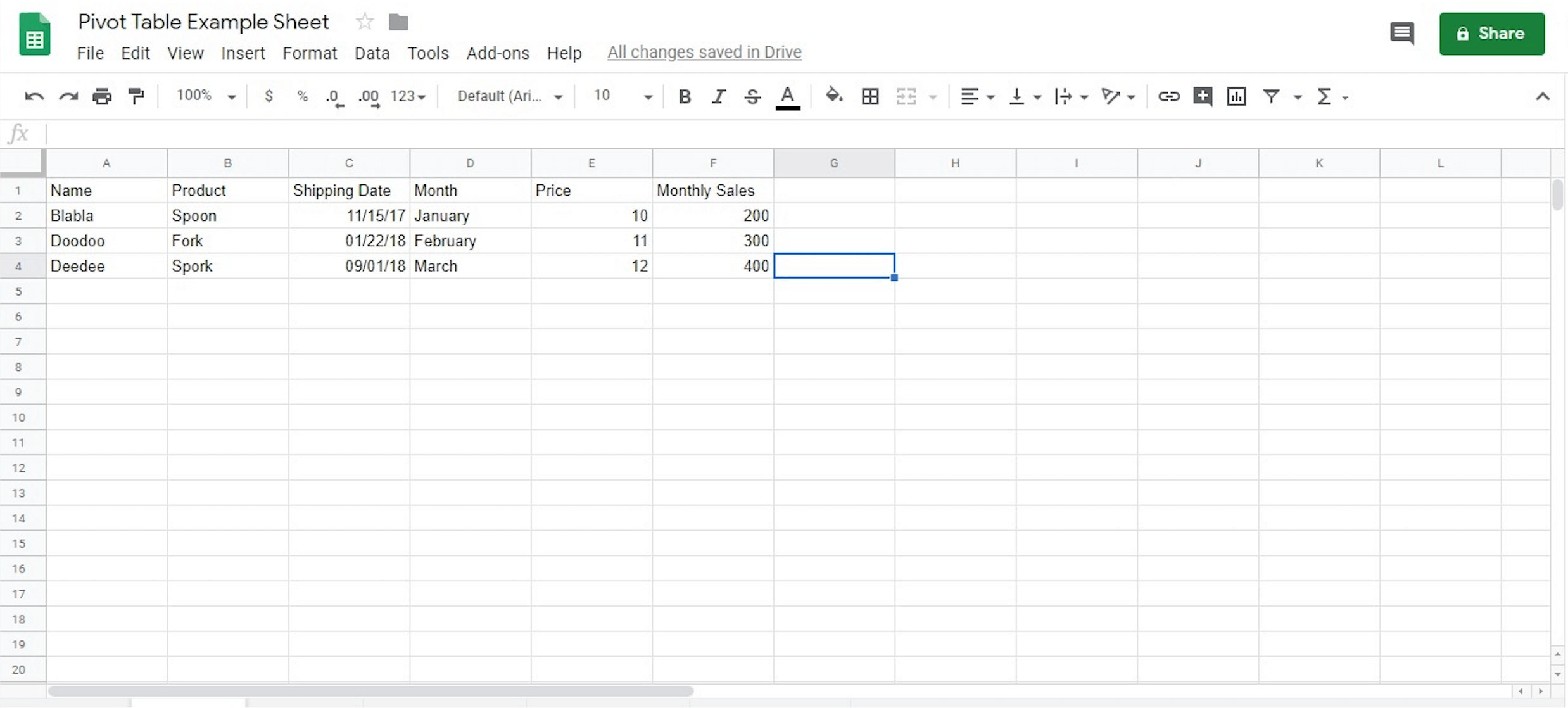
Open an Existing Google Sheet or Create a New
Pivot tables Google Sheets features require an existing sheet to work off of. So you either need to open the document that you already have on hand or create one from scratch. The image below shows just one simple example of a sheet that can be used to create the pivot tables using flat data.

-
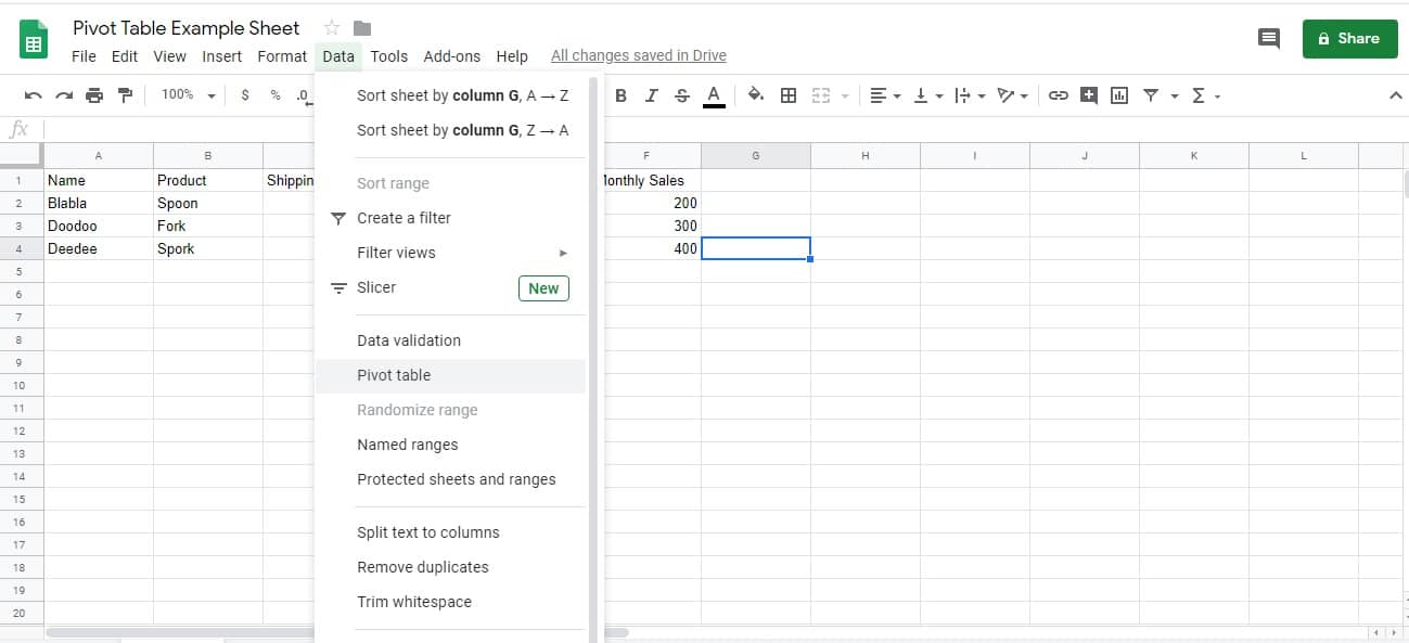
Create a Pivot Table
Once you have a sheet to work with, you can click Data on the toolbar and click Pivot Table on the dropdown options.

-
Select the Data to Include
After clicking the appropriate option, select New Sheet on the new window that pops out. After that, you will need to indicate the range of the data that you will include on the sheet. You can either do this manually or you can click on the Select Data Range prompt on the left of the input box.

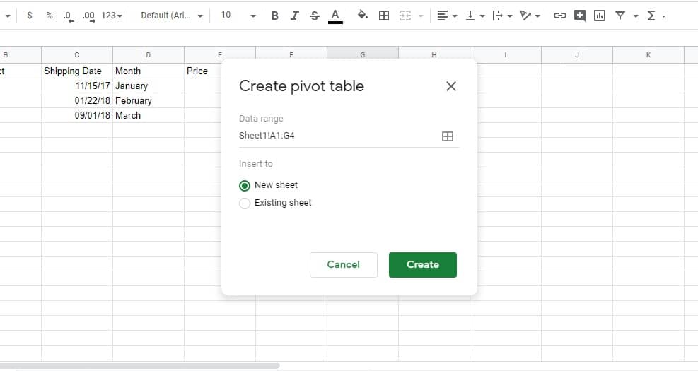
Once you click the command prompt, you will need to indicate the data you wish to include by highlighting them. -
Choosing Which Data to Include
Once you have created the pivot table, you should find yourself looking at the Pivot Table Editor. This is basically where you select which data sets you want to see using the options available.

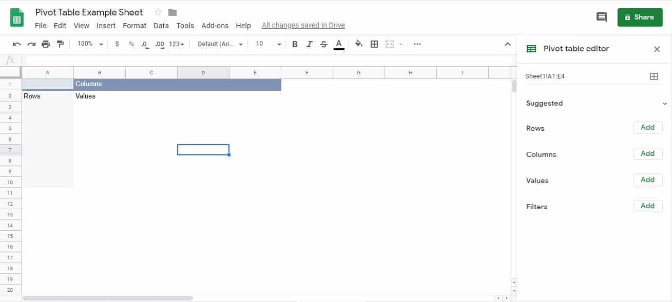
Through the options you are provided, you can choose which data sets go to which row or column, allowing you to see only the data sets that you are looking for. This is handy when you are creating a new report where the data come with their own dropdown options such as the example featured below. -
Customizing and Editing
Using the Pivot Table Editor, you can add or remove the data on the report you are trying to create as much as you want. This way, you will only present or see the details that you want, clearing away the clutter and giving you a clearer understanding of the information without additional distractions.
You can also scroll down the Pivot Table Editor to reach the Filter option where you can choose to hide certain data sets that you don’t want others to see without creating an entire new pivot table or sheet.
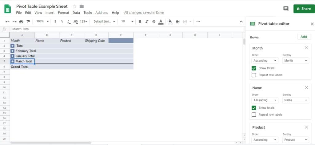
How to Refresh Pivot Tables in Google Sheets?
Refreshing the pivot table is really just about using the pivot table editor as you require. Alternatively, you could also go to the base sheet itself and add or remove any items that you might not need to show up on the pivot table. Both actions can result in the pivot table getting refreshed and updated to the version that you need.
Just take the before and after examples of pivot tables below where items are taken away:
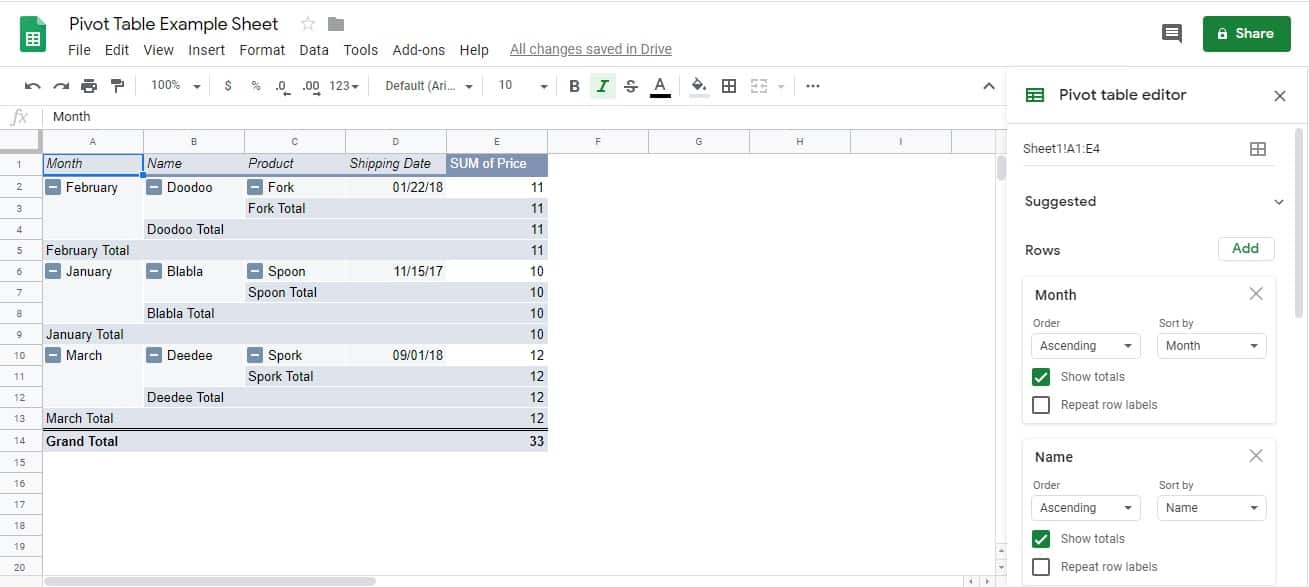
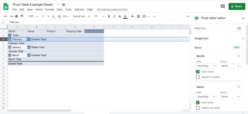
How to Group Pivot Tables by Month in Google Sheets?
If the goal is to group data sets together based on the months, it’s as easy as adding the Months rows right at the top. You just need the right column for the job where you include the months and then add it via the row section of the Pivot Table Editor.
You will then need to drag that new item right towards the top so that the table will be grouped based on the months. The images below should give you a pretty good idea of what this will look like.
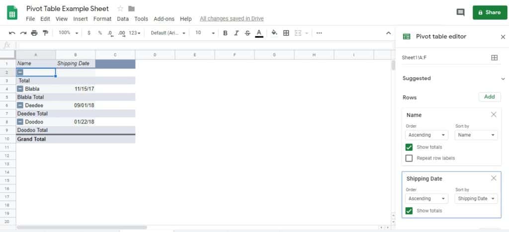
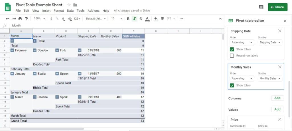
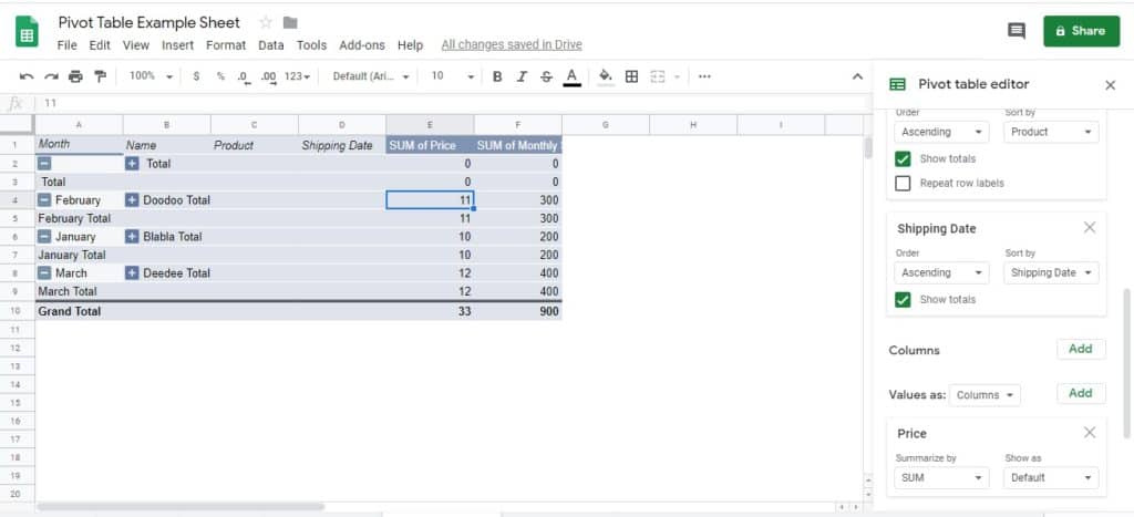
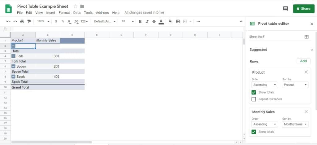
How to Sort in Pivot Tables?
Sorting in pivot tables is all about using the pivot table editor as needed. You add or remove the items that you want to feature as you see fit, exclude the items you don’t want to be visible by deleting them or using the filter, or dragging and dropping so that you can arrange which items show up first.
A lot of this will depend on what kind of report you are making and what you are trying to achieve. The same sheet can present different pictures based on the pivot table that you use. In the example below, you only have the product and the monthly sales.
In this next example, you only have the name and the shipping dates: