Google Sheets has a lot of neat functions that help make it one of the most convenient spreadsheet tools around and the ability to lock cells is one of them. You don’t want others to be able to mess around with your report without your permission, after all. The question now is how you will do that.
In this piece, this is exactly what we will go through one step at a time. We will also cover such topics as why you would want to lock cells, in the first place, as well as why you would want to use Google Sheets for making your reports.
In simple terms, locking cells is basically making sure that only those who are authorized to tamper with the data held by that particular part of the spreadsheet can actually do so. This can be done in a variety of different ways depending on the spreadsheet tool that is being used.
Now, it is important to note that this is different from other methods of protecting spreadsheet documents against tampering. For example, it is a more specific option of making sure that a particular figure is not messed with than something like locking the entire document.
In those kinds of cases, not only the cells, but the entire report itself will be inaccessible. Then there are cases with tools like Google Sheet where access can be shared. However, there are ways to make that access quite limited where you as the original owner will dispense editing privileges, as you please.
In the case of locking cells, though, only that particular cell will be inaccessible. The rest of the sheet can be free game, but not the specific cells that are locked.
On the matter of why locking cells even matters, it’s all about maintaining the accuracy, reliability, and quality of the report. It prevents any incident of inaccurate data getting introduced into the report whether through accidental interactions or intentional sabotage.
This is particularly important in cases where the report itself will play a role in the future of a large company. Even mistakes in the decimals can render a report disastrous for a corporation’s bottom line and an added zero is quite easy to overlook if the spreadsheet’s data set is already quite extensive.
Simply put, it is a means of protecting your sensitive report and the information that is held in it. If nothing else, it can help make sure that even you will not end up messing it up if you are not paying attention. After all, it does not take a malicious individual to make a report useless since it can just as easily be due to human error.
Step by Step: How to Lock Cells In Google Sheets
Time needed: 5 minutes.
-
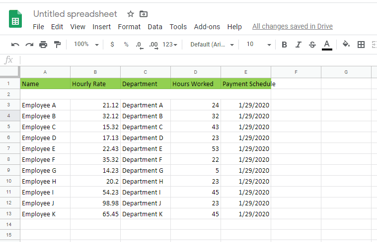
Open a Google Sheet Doc
Whether you open an existing Google Sheet document or create a new one, you can go with either route. Just don’t choose an important report for the former since you might end up messing up.

-
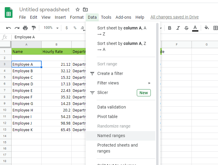
Click Named Range
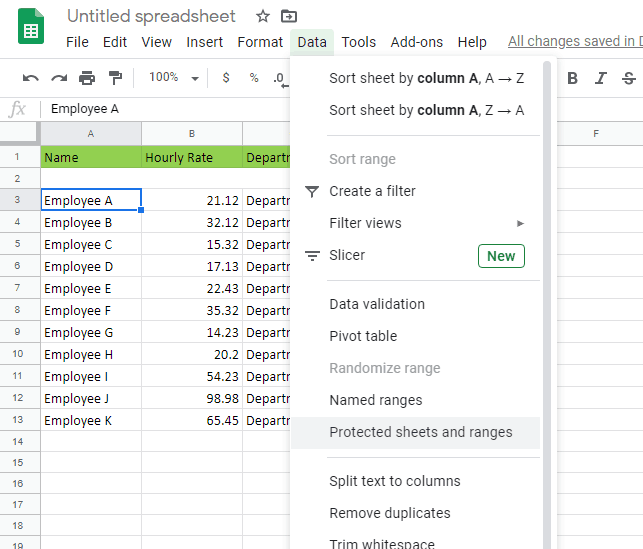
Once the document is opened, you can click on the Data menu on the taskbar and then click the Named ranges option in the dropdown.

-
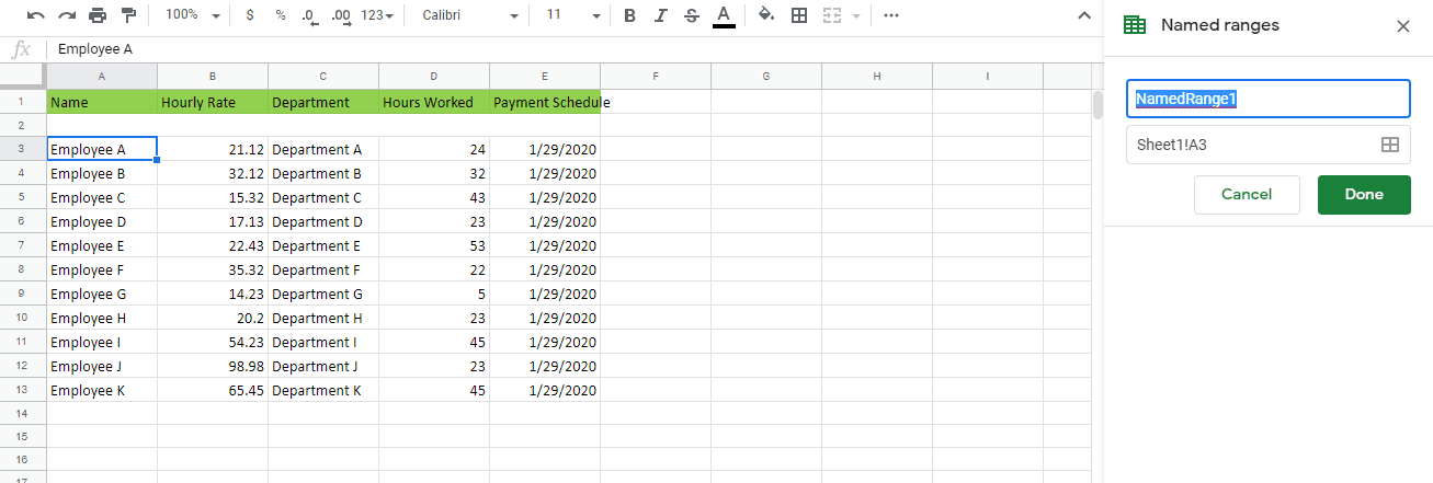
Set Named Range
Once the Named Ranges editor comes out, you can set the name of the cell that you are trying to lock and which cell it should be.

-
Click Protected Sheets and Named Ranges
After setting the name of the cell, you can then click on the Data menu on the taskbar again and this time, you can click the Protected Sheets and Named Ranges option on the dropdown menu.

-
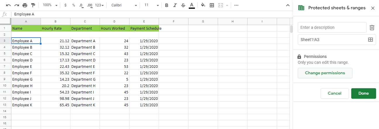
Set Protected Sheets and Named Ranges
Once the Protected Sheets and Named Ranges editor is out, you can select the cell that you want to lock and then click the Change Permissions button.

-
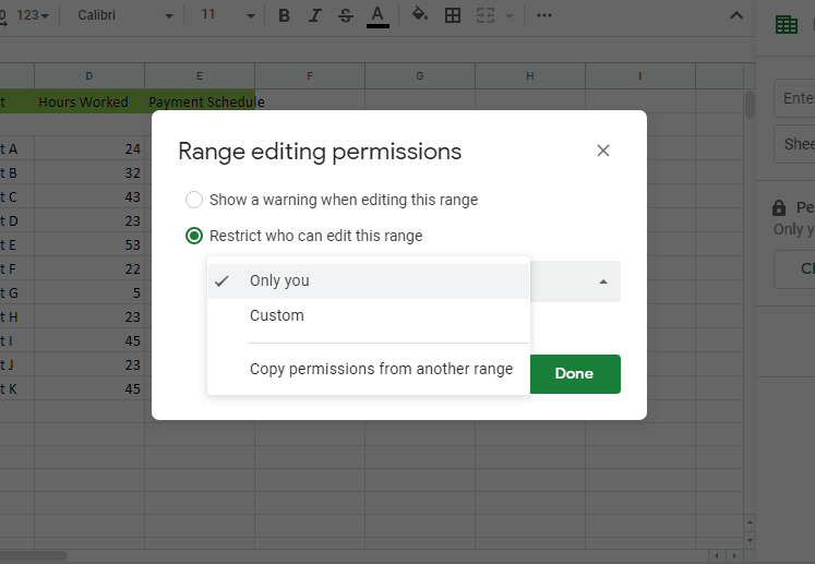
Set Permission
After clicking the Change Permissions button, you the appropriate window will pop out where you can then set who can access the cell.