There are many tools available on Google Sheets to help users create the very best reports that they can, especially when the report needs to be presented to some very important people. One of them is the ability to affect the color of the background and texts of a row or column of cells if they meet specific conditions. This is what conditional formatting is.
You are basically looking at the ability to direct attention to a particular section of your report where a very specific set of data is the most important to focus on. You can be the one to decide what the criteria of this should be and how you can best take advantage of it through the colors of the highlights that you are going to use.
Steps for Using Conditional Formatting
Time needed: 5 minutes.
-
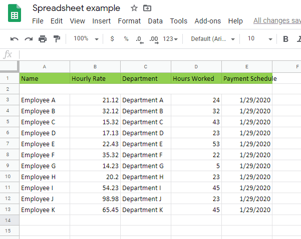
Open Google Sheet Doc
The first step is to open an appropriate Google Sheet doc that you will be using for your conditional formatting. It does not have to be an existing one since you can just create a dummy sheet to practice on. For the sake of playing it safe, you might want to do just that. Then again, removing the function is not all that difficult, so it’s not a big deal if you mess up.

-
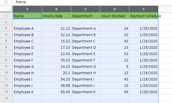
Highlight Cells
Next, you need to highlight the cells that you will be applying the function to. In many cases, highlighting the entire sheet works best.

-
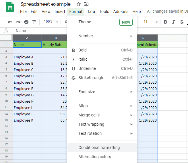
Click Conditional Formatting
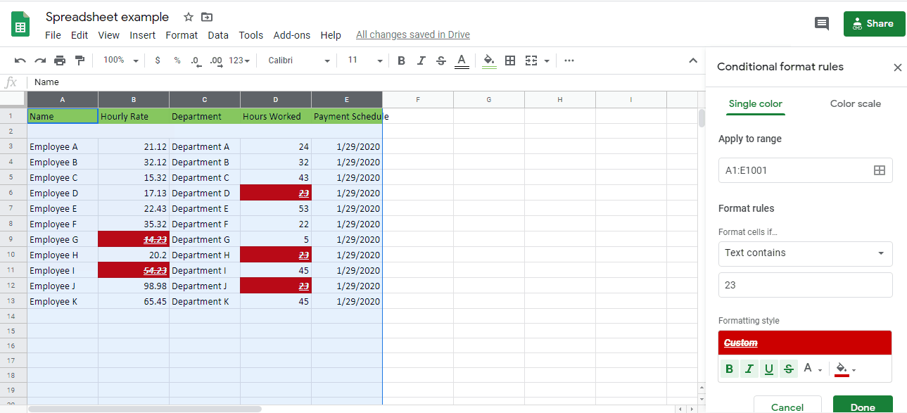
You then need to click the Format menu on the toolbar and then click Conditional Formatting on the dropdown menu where a pop-up will appear.

-
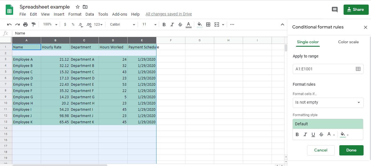
Indicate Value
On the pop-up editing menu that appears, you can change which cells you wish to highlight and what kinds of effects you want to occur.

-
Customize
You can choose to go with the generic options with the background colors or the font colors. However, you can also customize them by choosing bold, italic, underline, and more.

-
Finish up
Once you are done, you just need to finish up.

What is Conditional Formatting?
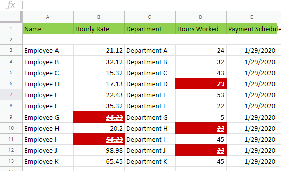
In essence, conditional formatting is the application of specific instructions on a series of cells so that you can bring about a particular effect if they meet the criteria that you set down. Simply put, you can create a report where every single time the cells that you have chosen hit a fit a particular profile, it will immediately jump out at those reading it.
The effects are typically limited to highlighting the cells’ background colors or the colors of the fonts. However, you can also customize this so that the values in the particular cells that are being highlighted will be bolded, will be underlined, will be in italic, and several other special effects that will make the presentation come alive.
Now, it should be noted here that the particular cells that will be highlighted based on your particular conditions.and it will only be those cells that will be affected. This means that you can apply the conditional formatting to the entire spreadsheet document and then make it so that only specific cells would jump out without having to select them one at a time.
Why Conditional Formatting Matters
Now, there are quite a few good reasons why you would want to make use of conditional formatting whenever you are making a report and these basically boil down to presentation.
That is to say, you can make quite a good impression using this function, which is always a good thing if you are talking to some industry bigwigs about stuff that they themselves should know like the back of their hands.
Of course, this is not just about presenting a solid report to superiors, either. It can also be about providing you or someone else more context about what you are working on. This can also be an immensely helpful feature when you are sharing your work with someone else or when you are working on a single spreadsheet as a group.
Just to make the whole thing clearer, though, just take a look at the following benefits that this function can afford you.
-
Professional Presentation – If you are going to make a presentation, you might as well make it look as professional as possible. That is to say, you make it as easy as possible for your audience to understand what you are talking about regardless of how complicated it actually is.
Being able to indicate specific cells that suit specific sets of data for your convenience will do exactly this. Your audience will not only be able to follow along as you are talking, but it will also assist you in remembering what you are talking about, in the first place. - Ease of Highlighting – Highlighting cells is just par for the course when using a spreadsheet. Through conditional formatting, it becomes a lot easier to do this without having to find each and every relevant cell to highlight them one at a time. Not only does it save you time, but it’s also downright convenient.
- Faster Indication of Value – If you are looking for certain sets of value, you can just input that as you please. It will make finding them on the sheet a lot easier and you won’t have to keep scrolling every which way.
- Grabbing Attention – Naturally, you want to draw your audience’s attention to specific parts of your report. This is a good way to do that, as well as to emphasize exactly what you want them to focus on.
- Indicating when Editing – When you are looking at the spreadsheet of a subordinate or someone you are working with, this function can be a great way to indicate what needs changing or if you yourself are marking them for future editing.
- Highlighting for Feedback – If you are working with a group for your report, it becomes easier to provide corrections, comments, and feedback using this method. Just highlight the cells in question and tag them as you see fit.