Vlookups can easily be used for Dropdown Lists in Google Sheets. If you don’t know what Vlookups are about, or how to use them, check our full guide here.
Time needed: 3 minutes.
On the matter of creating a dropdown list using the Vlookup function, simply follow these steps:
-
Data Validation
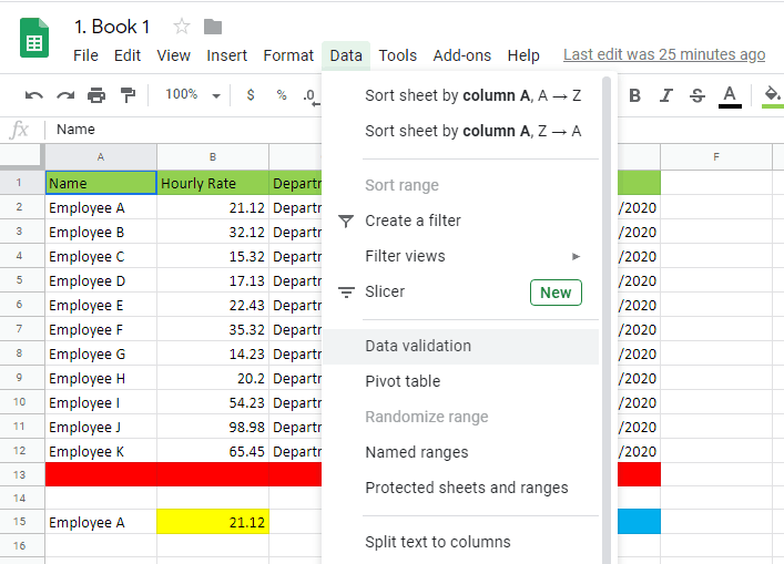
Using the same file as the one we opened in our vlookup guide, go to the Data menu on the menu toolbar, select the Data Validation dropdown tool, and click Data Validation.

-
Set Parameters for data validation
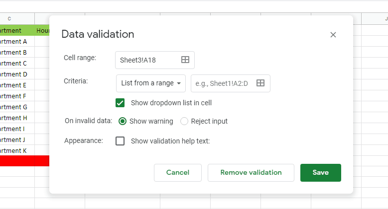
Once the pop-up window for the Data Validation comes out, you can set the parameters that you want. For this example, in the Criteria section, you can choose List From a Range. From there, you can click on the Cell box to indicate the column you will include. In this example, we will be using the Name column.

-
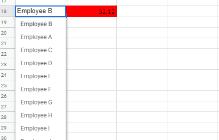
Dropdown
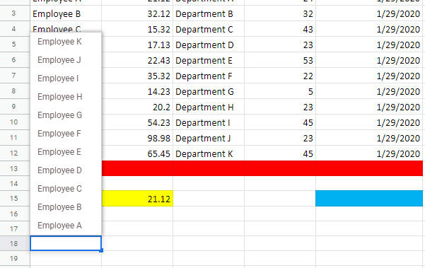
This will net you a dropdown list, much like what you will find in the image below.

-
Input Parameters
With that done, all you need to do is include the Vlookup function and you basically do it by following the steps in the earlier section of this guide. Only this time, you will use the dropdown Name list as the value.

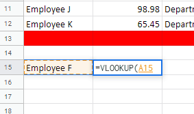
-
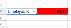
Name list as the value
What you will then get is a Vlookup function that you can change at will by simply switching between the items in the dropdown list.

-
Simply switching
Now you can simply select the option you like based on your Vlookup.