You might have heard of this function of Google Sheets called Vlookup but are a little unclear as to what exactly it is. More to the point, you don’t know how to use it or what it can even be used for. You’re in luck, then, because those are the topics that we will be covering today.
We will go through the main functions of Vlookup, its potential uses for any task you might assign to it, and what you can do if something goes wrong. Just to keep things brief, we won’t go into the more nitty-gritty details that might take a more in-depth explanation to understand. Today’s goal is to simply get you acquainted enough with the Google Sheets feature so that you will be able to make use of it.
What is Vlookup?
Vlookup stands for “vertical lookup” and it is a function that is already built into Google Sheets with the purpose of organizing data into specific columns. It is basically a means of putting together specific data in a file that you might be looking for under a particular category while removing the rest, which could prove distracting.
The data could come in the vein of such examples as names, dates, duration, departments, and so on. Doing this basically makes the report cleaner and leaves less room for confusion.
Steps for Using Vlookup
Time needed: 15 minutes.
The best way to understand Vlookup is to know how to use it in the first place. The steps below should help with that, which should make your Google Sheets reports much more organized.
-
Open or Create a New Google Sheets Document
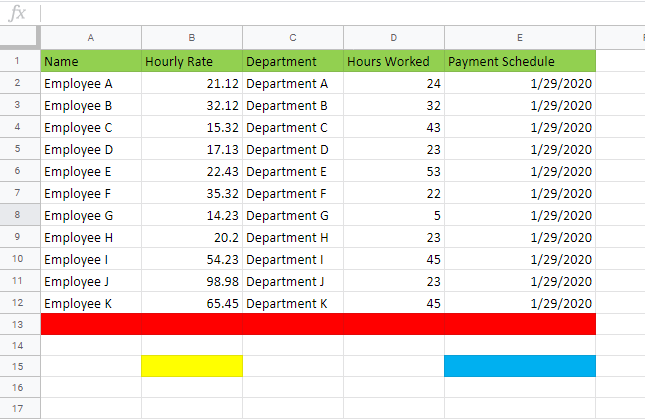
The first step is to open the document that you are going to use for creating your Vlookup function. It needs to have the necessary parameters such as the point of reference, figures, and scope. Without that, the Vlookup function will not know what to look for.
It would also help if the parameters were organized sensibly beforehand. This means that the data in the columns must follow a logical setup. This will help make sure that there will be fewer issues regarding the value that the function will retrieve.
-
Set the Value you are looking for
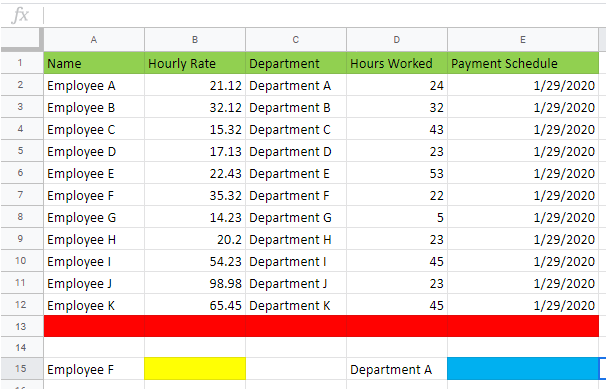
With that done, you will need to set the value that you are looking for in a separate cell. You need to make sure that the value actually reflects the ones that are already in the sheet. This will make sure that you are going to get what you want if you are looking for an exact match.
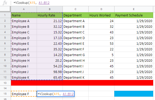
In our example, we want to get the Value “Hourly Rate” for “Employee F” into B15.
-
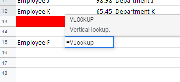
Input the Parameters
Once you are done setting the value, it’s time to input the parameters that you are looking for. To start with, you need to select a cell and type in “=VLOOKUP”, preferably next to the value that you have set.

-
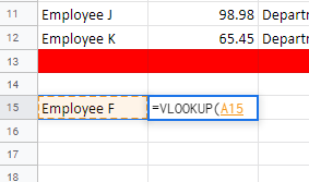
Indicate Cells
Then, you need to set an open parenthesis before proceeding to indicate the cell of the value that you set.

-
Input Range
You then need to type a comma before proceeding to indicate the columns that will serve as the range of data where the Vlookup functional will be pulling value from by highlighting them.

-
Input Number of Columns
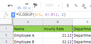
After another comma, you need to indicate how many columns are via the input bar.

-
Set True or False
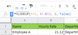
The next step is to indicate if you want to get an exact match for the parameters that you have set or not. If you want an exact match, you need to type in FALSE and if you don’t want an exact match, you type in TRUE.

-
Hit ENTER
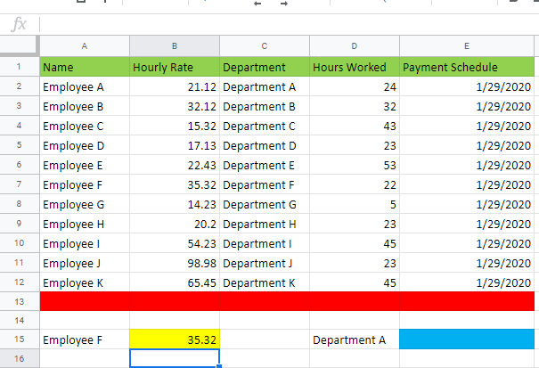
After making sure that all of the parameters are actually correct, you just need to hit ENTER and you should get the data that you need with the Vlookup function. You can try messing around with the results by changing the value to others in the same column to make sure that you are getting accurate results.

Vlookup and Other Features or Files
Whenever the #N/A error pops up when you are using the Vlookup function, you can actually make use of the IFERROR function to address the problem. It’s basically where you include the IFERROR function right before the VLOOKUP one so that you can find what the problem is.
Doing so will then alert you to the issue that is causing the problem to begin with so that you can fix it from there.
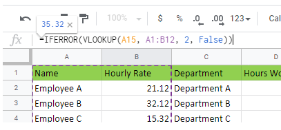
Example: =IFERROR( YOUR VLOOKUP )
On the matter of using the Vlookup function if you have two or more Google Sheets workbooks open, you basically just need to switch documents to indicate the value you are going for. You basically just type in the formula in the first document and then switch to the other include the rest of the arguments.
Common Issues with Vlookup
While the Vlookup function is handy, there can be a few issues with it that can affect a user’s experience with it. However, most of these issues actually stem from misunderstandings regarding the feature and mistakes by inexperienced users. To help avoid that, here are some examples of mistakes worth noting:
- No Value indicated – failure to indicate the value that the Vlookup function is supposed to base on.
- Wrong number of columns – the number of columns indicated in the parameters must be accurate or it will cause issues.
- Failing to indicate match – you must type False if you want an exact match or True if you don’t, and forgoing this can cause the function to malfunction.
- Exact space – the parameters are only meant to have one space between them and adding more can lead to errors.